Get Started

Quickstart

In this vignette we will show how to get started with mlr3torch by training a simple neural network on a tabular regression problem. We assume that you are familiar with the mlr3 framework, see e.g. the mlr3 book. As a first example, we will train a simple multi-layer perceptron (MLP) on the well-known “mtcars” task, where the goal is to predict the miles per galleon (‘mpg’) of cars. This architecture comes as a predfined learner with mlr3torch, but you can also easily create new network architectures, see the Neural Networks as Graphs vignette for a detailed introduoduion. We first set a seed for reproducibility, load the library and construct the task.

set.seed(314)
library(mlr3torch)
task = tsk("mtcars")
task$head()
#>      mpg    am  carb   cyl  disp  drat  gear    hp  qsec    vs    wt
#>    <num> <num> <num> <num> <num> <num> <num> <num> <num> <num> <num>
#> 1:  21.0     1     4     6   160  3.90     4   110 16.46     0 2.620
#> 2:  21.0     1     4     6   160  3.90     4   110 17.02     0 2.875
#> 3:  22.8     1     1     4   108  3.85     4    93 18.61     1 2.320
#> 4:  21.4     0     1     6   258  3.08     3   110 19.44     1 3.215
#> 5:  18.7     0     2     8   360  3.15     3   175 17.02     0 3.440
#> 6:  18.1     0     1     6   225  2.76     3   105 20.22     1 3.460

Learners in mlr3torch work very similary to other mlr3 learners. Below, we construct a simple multi layer perceptron for regression. We do this as usual by calling lrn() and configuring the parameters: We use two hidden layers with 50 neurons, For training, we set the batch size to 32, the number of training epochs to 30 and the device to "cpu". For a complete description of the available parameters see ?mlr3torch::LearnerTorchMLP.

mlp = lrn("regr.mlp",
  # architecture parameters
  neurons = c(50, 50),
  # training arguments
  batch_size = 32, epochs = 30, device = "cpu"
)
mlp
#> <LearnerTorchMLP[regr]:regr.mlp>: My Little Powny
#> * Model: -
#> * Parameters: epochs=30, device=cpu, num_threads=1, seed=random,
#>   eval_freq=1, measures_train=<list>, measures_valid=<list>,
#>   patience=0, min_delta=0, batch_size=32, neurons=50,50, p=0.5,
#>   activation=<nn_relu>, activation_args=<list>
#> * Validate: NULL
#> * Packages: mlr3, mlr3torch, torch
#> * Predict Types:  [response]
#> * Feature Types: integer, numeric, lazy_tensor
#> * Properties: internal_tuning, marshal, validation
#> * Optimizer: adam
#> * Loss: mse
#> * Callbacks: -

We can use this learner for training and prediction just like any other regression learner. Below, we split the observations into a training and test set, train the learner on the training set and create predictions for the test set. Finally, we compute the mean squared error of the predictions.

# Split the obersevations into training and test set
splits = partition(task)
# Train the learner on the train set
mlp$train(task, row_ids = splits$train)
# Predict the test set
prediction = mlp$predict(task, row_ids = splits$test)
# Compute the mse
prediction$score(msr("regr.mse"))
#> regr.mse 
#>  283.838

Configuring a Learner

Although torch learners are quite like other mlr3 learners, there are some differences. One is that all LearnerTorch classes have construction arguments, i.e. torch learners are more modular than other learners. While learners are free to implement their own construction arguments, there are some that are common to all torch learners, namely the loss, optimizer and callbacks. Each of these object can have their own parameters that are included in the LearnerTorch’s parameter set.

In the previous example, we did not specify any of these explicitly and used the default values, which was the Adam optimizer, MSE as the loss and no callbacks. We will now show how to configure these three aspects of a learner through the mlr3torch::TorchOptimizer, mlr3torch::TorchLoss, and mlr3torch::TorchCallback classes.

Loss

The loss function, also known as the objective function or cost function, measures the discrepancy between the predicted output and the true output. It quantifies how well the model is performing during training. The R package torch, which underpins the mlr3torch framework, already provides a number of predefined loss functions such as the Mean Squared Error (nn_mse_loss), the Mean Absolute Error (nn_l1_loss), or the cross entropy loss (nn_cross_entropy_loss). In mlr3torch, we represent loss functions using the mlr3torch::TorchLoss class. It provides a thin wrapper around the torch loss functions and annotates them with meta information, most importantly a paradox::ParamSet that allows to configure the loss function. Such an object can be constructed using t_loss(<key>). Below, we construct the L1 loss function, which is also known as Mean Absolute Error (MAE). The printed output below informs us about the wrapped loss function (nn_l1_loss), the configured parameters, the packages it depends on and for which task types it can be used.

l1 = t_loss("l1")
l1
#> <TorchLoss:l1> Absolute Error
#> * Generator: nn_l1_loss
#> * Parameters: list()
#> * Packages: torch,mlr3torch
#> * Task Types: regr

Its ParamSet contains only one parameter, namely reduction, which specifies how the loss is reduced over the batch.

# the paradox::ParamSet of the loss
l1$param_set
#> <ParamSet(1)>
#>           id    class lower upper nlevels default  value
#>       <char>   <char> <num> <num>   <num>  <list> <list>
#> 1: reduction ParamFct    NA    NA       2    mean [NULL]

The wrapped loss module generator is accessible through the slot $generator.

l1$generator
#> <nn_l1_loss> object generator
#>   Inherits from: <inherit>
#>   Public:
#>     .classes: nn_l1_loss nn_loss nn_module
#>     initialize: function (reduction = "mean") 
#>     forward: function (input, target) 
#>     clone: function (deep = FALSE, ..., replace_values = TRUE) 
#>   Private:
#>     .__clone_r6__: function (deep = FALSE) 
#>   Parent env: <environment: 0x563a5a08a0a8>
#>   Locked objects: FALSE
#>   Locked class: FALSE
#>   Portable: TRUE

We can pass the TorchLoss as the argument loss during initialization of the learner. The parameters of the loss are added to the learner’s ParamSet, prefixed with "loss.".

mlp_l1 = lrn("regr.mlp", loss = l1)
mlp_l1$param_set$values$loss.reduction
#> NULL

All predefined loss functions are stored in the mlr3torch_losses dictionary, from which they can be retrieved using t_loss(<key>).

mlr3torch_losses
#> <DictionaryMlr3torchLosses> with 3 stored values
#> Keys: cross_entropy, l1, mse

Optimizer

The optimizer determines how the model’s weights are updated based on the calculated loss. It adjusts the parameters of the model to minimize the loss function, optimizing the model’s performance. Optimizers work analogous to loss functions, i.e. mlr3torch provides a thin wrapper – the TorchOptimizer class – around the optimizers such as Adam (optim_adam) or SGD (optim_sgd). TorchLoss objects can be constructed using t_opt(<key>). For optimizers, the associated ParamSet is more interesting as we see below:

sgd = t_opt("sgd")
sgd
#> <TorchOptimizer:sgd> Stochastic Gradient Descent
#> * Generator: optim_sgd
#> * Parameters: list()
#> * Packages: torch,mlr3torch

sgd$param_set
#> <ParamSet(5)>
#>              id    class lower upper nlevels        default  value
#>          <char>   <char> <num> <num>   <num>         <list> <list>
#> 1:           lr ParamDbl     0   Inf     Inf <NoDefault[0]> [NULL]
#> 2:     momentum ParamDbl     0     1     Inf              0 [NULL]
#> 3:    dampening ParamDbl     0     1     Inf              0 [NULL]
#> 4: weight_decay ParamDbl     0     1     Inf              0 [NULL]
#> 5:     nesterov ParamLgl    NA    NA       2          FALSE [NULL]

The wrapped torch optimizer can be accessed through the slot generator.

Parameters of TorchOptimizer (but also TorchLoss and TorchCallback) can be set in the usual mlr3 way, i.e. either during construction, or afterwards using the $set_values() method of the parameter set.

sgd$param_set$set_values(
  lr = 0.5, # increase learning rate
  nesterov = FALSE # no nesterov momentum
)

Below we see that the optimizer’s parameters are added to the learner’s ParamSet (prefixed with "opt.") and that the values are set to the values we specified.

mlp_sgd = lrn("regr.mlp", optimizer = sgd)
as.data.table(mlp_sgd$param_set)[
  startsWith(id, "opt.")][[1L]]
#> [1] "opt.lr"           "opt.momentum"     "opt.dampening"    "opt.weight_decay"
#> [5] "opt.nesterov"
mlp_sgd$param_set$values[c("opt.lr", "opt.nesterov")]
#> $opt.lr
#> [1] 0.5
#> 
#> $opt.nesterov
#> [1] FALSE

By exposing the optimizer’s parameters, they can be conveniently tuned using mlr3tuning.

All available optimizers are stored in the mlr3torch_optimizers dictionary.

mlr3torch_optimizers
#> <DictionaryMlr3torchOptimizers> with 7 stored values
#> Keys: adadelta, adagrad, adam, asgd, rmsprop, rprop, sgd

Callbacks

The third important configuration option are callbacks which allow to customize the training process. This allows saving model checkpoints, logging metrics, or implementing custom functionality for specific training scenarios. For a tutorial on how to implement a custom callback, see the Custom Callbacks vignette. Here, we will only show how to use predefined callbacks. Below, we retrieve the "history" callback using t_clbk(), which has no parameters and merely saves the training and validation history in the learner so it can be accessed afterwards.

history = t_clbk("history")
history
#> <TorchCallback:history> History
#> * Generator: CallbackSetHistory
#> * Parameters: list()
#> * Packages: mlr3torch,torch

If we wanted to learn about what the callback does, we can access the help page of the wrapped object using the $help() method. Note that this is also possible for the loss and optimizer.

history$help()

All predefined callbacks are stored in the mlr3torch_callbacks dictionary.

mlr3torch_callbacks
#> <DictionaryMlr3torchCallbacks> with 3 stored values
#> Keys: checkpoint, history, progress

Putting it Together

We now define our customized MLP learner using the loss, optimizer and callback we have just covered. To keep track of the performance, we use 30% of the training data for validation and evaluate it using the MAE Measure. Note that the mearures_valid and measures_train parameters of LearnerTorch take common mlr3::Measures, whereas the loss function must be a TorchLoss.

mlp_custom = lrn("regr.mlp",
  # construction arguments
  optimizer = sgd, loss = l1, callbacks = history,
  # scores to keep track of
  measures_valid = msr("regr.mae"),
  # other parameters are left as-is:
  # architecture
  neurons = c(50, 50),
  # training arguments
  batch_size = 32, epochs = 30, device = "cpu",
  # validation proportion
  validate = 0.3
)

mlp_custom
#> <LearnerTorchMLP[regr]:regr.mlp>: My Little Powny
#> * Model: -
#> * Parameters: epochs=30, device=cpu, num_threads=1, seed=random,
#>   eval_freq=1, measures_train=<list>,
#>   measures_valid=<MeasureRegrSimple>, patience=0, min_delta=0,
#>   batch_size=32, neurons=50,50, p=0.5, activation=<nn_relu>,
#>   activation_args=<list>, opt.lr=0.5, opt.nesterov=FALSE
#> * Validate: 0.3
#> * Packages: mlr3, mlr3torch, torch
#> * Predict Types:  [response]
#> * Feature Types: integer, numeric, lazy_tensor
#> * Properties: internal_tuning, marshal, validation
#> * Optimizer: sgd
#> * Loss: l1
#> * Callbacks: history

We now train the learner on the “mtcars” task again and use the same train-test split as before.

mlp_custom$train(task, row_ids = splits$train)
prediction_custom = mlp_custom$predict(task, row_ids = splits$test)

Below we make predictions on the unseen test data and compare the scores. Because we directly optimized the L1 (aka MAE) loss and tweaked the learning rate, our configured mlp_custom learner has a lower MAE than the default mlp learner.

prediction_custom$score(msr("regr.mae"))
#> regr.mae 
#> 7.122375
prediction$score(msr("regr.mae"))
#> regr.mae 
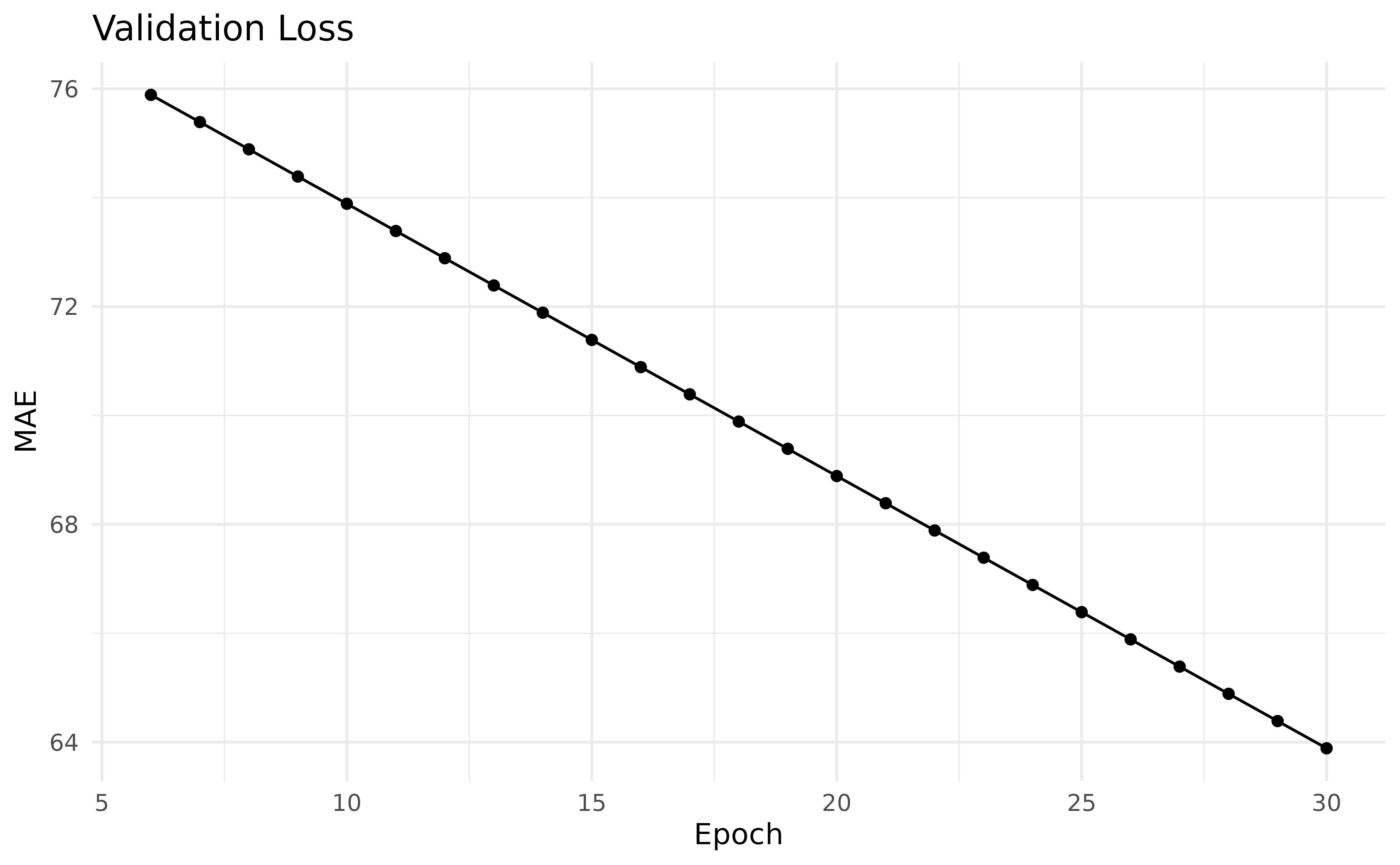
#> 15.27983

Because we configured the learner to use the history callback, we can find the validation history in its $model slot:

head(mlp_custom$model$callbacks$history$valid)
#>    epoch     regr.mae
#>    <num>        <num>
#> 1:     1 1.777395e+04
#> 2:     2 3.955504e+08
#> 3:     3 1.143863e+04
#> 4:     4 1.792927e+01
#> 5:     5 1.759594e+01
#> 6:     6 1.726260e+01

The plot below shows it for the epochs 6 to 30.

Other important information that is stored in the Learner’s model is the $network, which is the underlying nn_module. For a full description of the model, see ?LearnerTorch.