Lazy Tensor

This vignette introduces the lazy_tensor class, which is a vector type that can be used to lazily represent torch tensors of arbitary dimensions. Among other things, it allows mlr3torch to work with images, which we will illustrate using the predefined MNIST task, which has one feature image of class "lazy_tensor". The images display the digits 0, …, 9, and the goal is to classify them correctly.

library(mlr3torch)

mnist = tsk("mnist")
mnist
#> <TaskClassif:mnist> (70000 x 2): MNIST Digit Classification
#> * Target: label
#> * Properties: multiclass
#> * Features (1):
#>   - lt (1): image

The name "lazy_tensor" stems from the fact, that the tensors are not necessarily stored in memory, as this is often impossible when working with large image datasets.
Therefore, we can easily access the data without any expensive data-loading. We see that the data contains one column label, which is the target variable, and an image which is the input feature.

mnist$head()
#> Processing...
#> Done!
#>     label           image
#>    <fctr>   <lazy_tensor>
#> 1:      5 <tnsr[1x28x28]>
#> 2:      0 <tnsr[1x28x28]>
#> 3:      4 <tnsr[1x28x28]>
#> 4:      1 <tnsr[1x28x28]>
#> 5:      9 <tnsr[1x28x28]>
#> 6:      2 <tnsr[1x28x28]>

If we wanted to obtain the actual tensors representing the images, we can do so by calling materialize(), which will return a list of torch_tensors, not necessarily all with the same shape. Here, we only show a slice of the tensor for readability.

lt = mnist$data(cols = "image")[[1L]]
materialize(lt[1])[[1]][1, 12:16, 12:16]
#> torch_tensor
#>  139  253  190    2    0
#>   11  190  253   70    0
#>    0   35  241  225  160
#>    0    0   81  240  253
#>    0    0    0   45  186
#> [ CPUFloatType{5,5} ]

If all elements have the same shape as is the case here, we could also obtain a single torch_tensor by specifying rbind = TRUE.

In order to train a Learner on a Task containing lazy_tensor columns it must support the lazy_tensor feature type, as is the case for the multi layer perceptron, which works both with numeric types, as well as the lazy_tensor.

mlp = lrn("classif.mlp",
  neurons = c(100, 100),
  epochs = 10, batch_size = 32
)
mlp
#> <LearnerTorchMLP[classif]:classif.mlp>: My Little Powny
#> * Model: -
#> * Parameters: epochs=10, device=auto, num_threads=1, seed=random,
#>   eval_freq=1, measures_train=<list>, measures_valid=<list>,
#>   patience=0, min_delta=0, batch_size=32, neurons=100,100, p=0.5,
#>   activation=<nn_relu>, activation_args=<list>
#> * Validate: NULL
#> * Packages: mlr3, mlr3torch, torch
#> * Predict Types:  [response], prob
#> * Feature Types: integer, numeric, lazy_tensor
#> * Properties: internal_tuning, marshal, multiclass, twoclass,
#>   validation
#> * Optimizer: adam
#> * Loss: cross_entropy
#> * Callbacks: -

However, because lazy_tensors also have a specific shape, we also must ensure that the shape of the lazy_tensor matches the expected input shape of the learner. The multi layer perceptron expects a 2d-tensor where the first dimension is the batch dimension. But above we have seen that this is not the case for MNIST, where each element has shape (1, 28, 28). Therefore, we need to flatten the lazy_tensor, which we here do using po("trafo_reshape"):

reshaper = po("trafo_reshape", shape = c(-1, 28 * 28))
mnist_flat = reshaper$train(list(mnist))[[1L]]
mnist_flat$head()
#>     label         image
#>    <fctr> <lazy_tensor>
#> 1:      5   <tnsr[784]>
#> 2:      0   <tnsr[784]>
#> 3:      4   <tnsr[784]>
#> 4:      1   <tnsr[784]>
#> 5:      9   <tnsr[784]>
#> 6:      2   <tnsr[784]>

Note that this does not actually reshape all the tensors in-memory, this will again only happen once materialize() is called.

We can now proceed to train the a simple multi-layer perceptron on the flattened mnist task:

mlp = lrn("classif.mlp",
  neurons = c(100, 100),
  epochs = 10, batch_size = 32
)
mlp$train(mnist_flat)

Creating a Lazy Tensor

Every lazy_tensor is built on top of a torch::dataset, so we here assume that you are familiar with it. For more information on how to create torch::datasets, we recommend reading the torch package documentation. The only additional restriction that we impose on the dataset is that it must have a .getitem or .getbatch method that returns a list of named tensors.

As an example, we will create a lazy_tensor of length 1000, whose elements are drawn from a uniform distribution over \([0, 1]\). While the data is stored in-memory in this example, this is not necessary and the $.getitem() method can e.g. load images from disk.

mydata = dataset(
  initialize = function() {
    self$x = runif(1000, -1, 1)
  },
  .getbatch = function(i) list(x = torch_tensor(self$x[i])$unsqueeze(2)),
  .length = function() 1000
)()

In order to create a lazy_tensor from mydata, we have to annotate the returned shapes of the dataset by passing a named list to dataset_shapes. The first dimension must be NA, as it is the batch dimension. We can also set a shape to NULL to indicate that it is unknown, i.e. it varies between elements.

lt = as_lazy_tensor(mydata, dataset_shapes = list(x = c(NA, 1)))
lt[1:5]
#> <ltnsr[5]>
#> [1] <tnsr[1]> <tnsr[1]> <tnsr[1]> <tnsr[1]> <tnsr[1]>

Note that in this case, because we implemented the .getbatch method, we could have even omitted specifying the dataset_shapes as they could have been auto-inferred.

We can convert this vector to a torch_tensor just like before:

materialize(lt[1:5], rbind = TRUE)
#> torch_tensor
#> -0.9852
#> -0.0672
#> -0.0044
#> -0.4205
#>  0.4658
#> [ CPUFloatType{5,1} ]

Because we added no preprocessing, this is the same as calling the $.getbatch() method on mydata and selecting the element x.

torch_equal(
  materialize(lt[1], rbind = TRUE),
  mydata$.getbatch(1)$x
)
#> [1] TRUE

We continue with creating an example task from lt, where the relationship between the x and y variable is polynomial. Note that the target variable, both for classification and regression, cannot be a lazy_tensor, but must be a factor or numeric respectively.

library(data.table)
x = mydata$x
y = 0.2 + 0.1 * x - 0.1 * x^2 - 0.3 * x^3 + 0.5 * x^4 + 0.5 * x^7 + 0.6 * x^11 + rnorm(length(mydata)) * 0.1
dt = data.table(y = y, x = lt)
task_poly = as_task_regr(dt, target = "y", id = "poly")
task_poly
#> <TaskRegr:poly> (1000 x 2)
#> * Target: y
#> * Properties: -
#> * Features (1):
#>   - lt (1): x

Below, we plot the data:

library(ggplot2)
ggplot(data = data.frame(x = x, y = y)) +
  geom_point(aes(x = x, y = y), alpha = 0.5)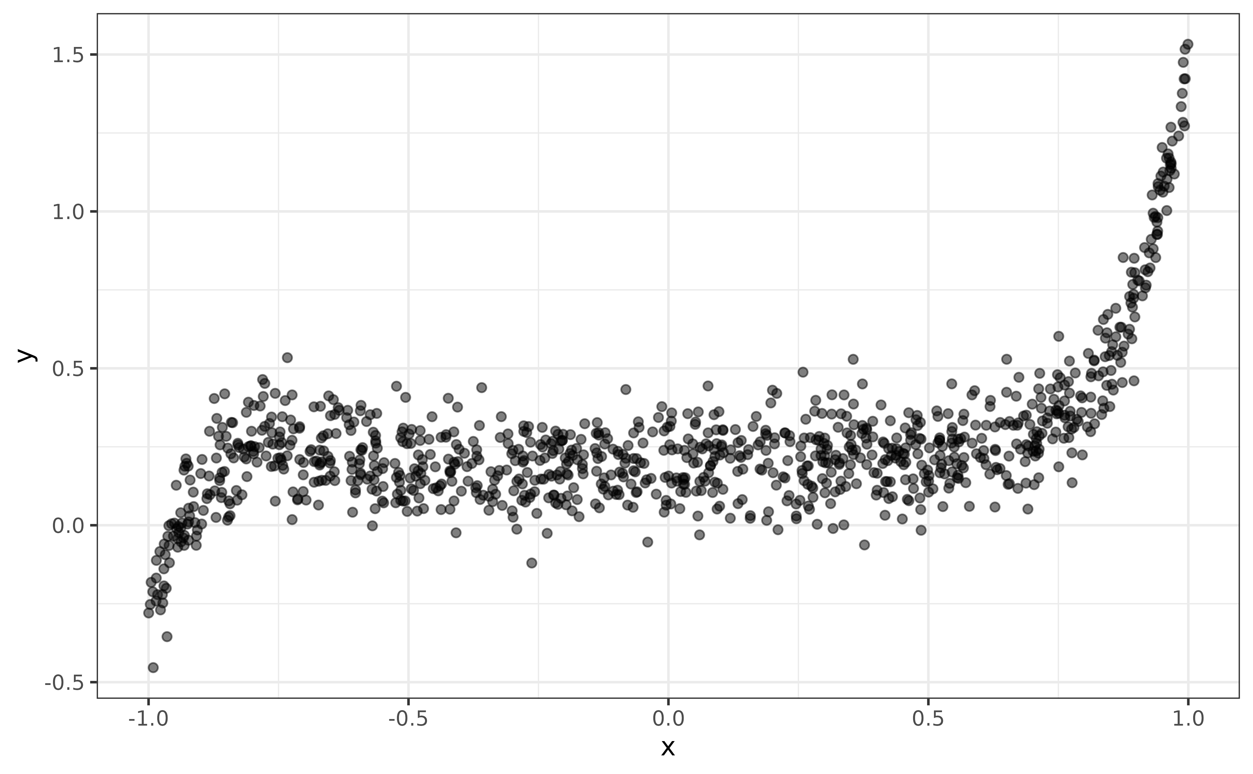

In the next section, we will create a custom PipeOp to fit a polynomial regression model.

Custom Preprocessing

In order to create a custom preprocessing operator for a lazy tensor, we have to create a new PipeOp class. To make this as convenient as possible, mlr3torch offters a pipeop_preproc_torch() function that we recommend using for this purpose. Its most important arguments are:

• id - Used as the default identifier of the PipeOp
• fn - The preprocessing function. By default, the first argument is assumed to be the torch_tensor and the remaining arguments will be part of the PipeOp’s parameter set.
• shapes_out - A function that returns the shapes of the output tensors given the input shapes. This can also be set to NULL for an unknown shape or to "infer" for auto-inference, see ?pipeop_preproc_torch for more information.

Below, we create a PipeOp, that transforms a vector x into a matrix \((x^{d_1} ..., x^{d_n})\), where \(d\) is the degrees parameter of the PipeOp.

PipeOpPreprocTorchPoly = pipeop_preproc_torch("poly",
  fn = function(x, degrees) {
    torch_cat(lapply(degrees, function(d) torch_pow(x, d)), dim = 2L)
  },
  shapes_out = "infer"
)

We can now create a new instance of this PipeOp by calling $new(), and we set the parameter degrees to those degrees that were used when simulating the data above. Further, we set the parameter stages, that is always available, to "both", which means that the preprocessing is applied during training and prediction. For data augmentation this can be set to "train".

po_poly = PipeOpPreprocTorchPoly$new()

po_poly$param_set$set_values(
  degrees = c(0, 1, 2, 3, 4, 7, 11),
  stages = "both"
)

To create our polynomial regression learner, we combine the polynomial preprocessor with a lrn("regr.mlp") with no hidden layer (i.e. a linear model) and train the learner on the task.

lrn_poly = as_learner(
  po_poly %>>% lrn("regr.mlp", batch_size = 256, epochs = 100,
  neurons = integer(0))
)

lrn_poly$train(task_poly)
pred = lrn_poly$predict(task_poly)

Below, we visualize the predictions and see that the model captured the non-linear relationship reasonably:

dt = melt(data.table(
  truth = pred$truth,
  response = pred$response,
  x = x),
  id.vars = "x", measure.vars = c("truth", "response")
)
dt$variable = factor(dt$variable, levels = c("truth", "response"))

ggplot(data = dt) +
  geom_point(aes(x = x, y = value, color = variable))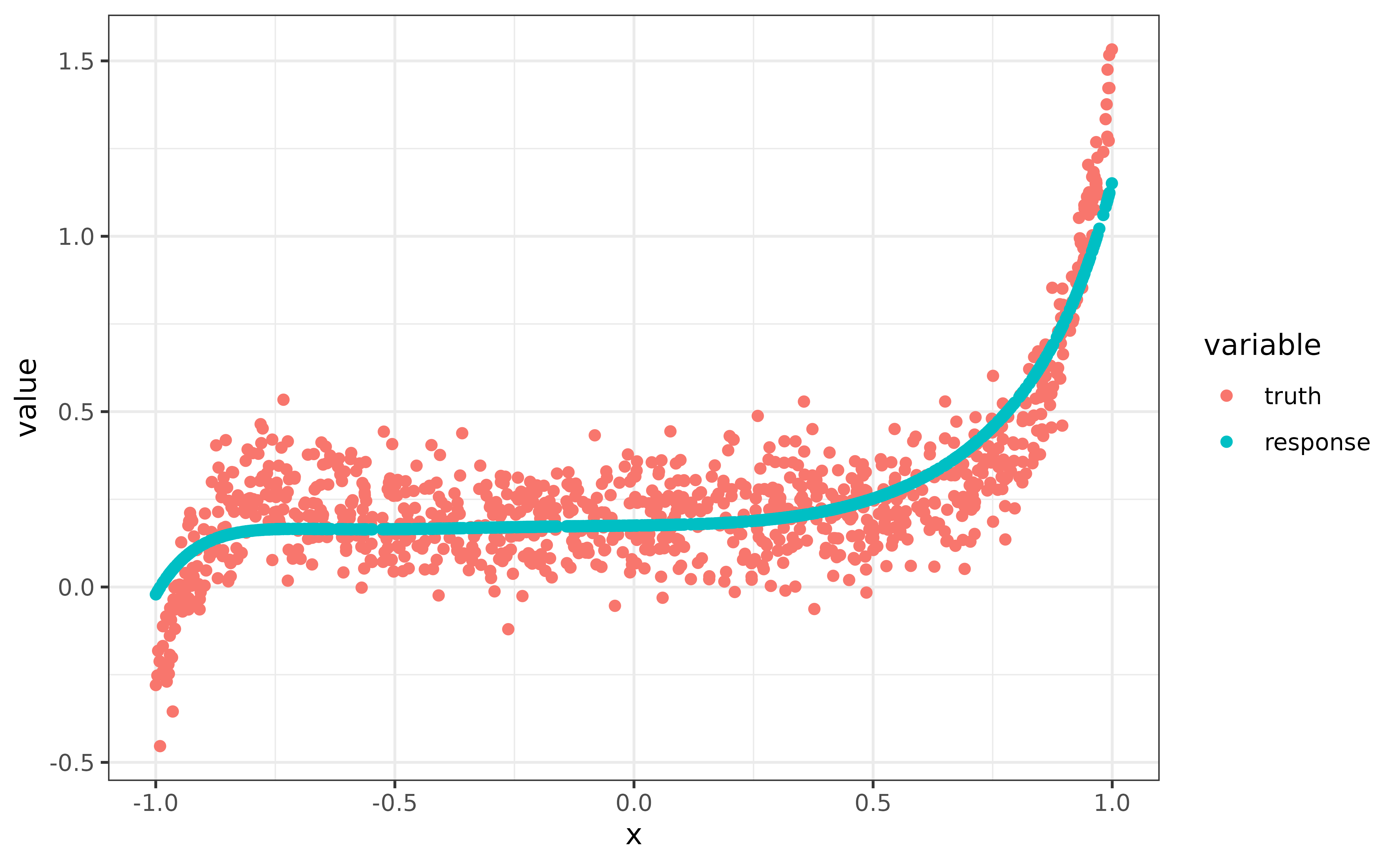

In the next section, we will briefly cover the implementation details of the lazy_tensor, which is not necessary to work with the data-type, so feel free to skip this part.

Digging Into Internals

Internally, the lazy_tensor vector uses the DataDescriptor class to represent the (possibly) preprocessed data. It is very similar to the ModelDescriptor class that is used to build up neural nerworks using PipeOpTorch objects. The DataDescriptor stores a torch::dataset, an mlr3pipelines::Graph and some metadata.

desc = DataDescriptor$new(
  dataset = mydata,
  dataset_shapes = list(x = c(NA, 1))
)

Per default, the preprocessing graph contains only a single PipOpNop that does nothing.

desc
#> <DataDescriptor: 1 ops>
#> * dataset_shapes: [x: (NA,1)]
#> * input_map: (x) -> Graph
#> * pointer: nop.ea1c6d.x.output
#> * shape: [(NA,1)]

The printed output of the data descriptor informs us about:

• The number of PipeOps contained in the preprocessing graph
• The output shapes of the dataset
• The input map, i.e. how the data is passed to the preprocessing graph, which is important when there are multiple inputs
• The pointer, which points to a specific channel of an output PipeOp. The output of this channel is the tensor represented by the DataDescriptor. Note that the id from the input po("nop") is randomly generated, which is needed to prevent id clashes then there are more than one input to the preprocessing graph.
• The shape, which is the shape of the tensor at position pointer

A lazy tensor can be constructed from an integer vector and a DataDescriptor. The integer vector specifies which element of the DataDescriptor the lazy_tensor contains. Below, the first two elements of the lazy_tensor vector represent the same element of the DataDescriptor, while the third element represents a different element. Note that all indices refer to the same DataDescriptor.

lt = lazy_tensor(desc, ids = c(1, 1, 2))
materialize(lt, rbind = TRUE)
#> torch_tensor
#> -0.9852
#> -0.9852
#> -0.0672
#> [ CPUFloatType{3,1} ]

Internally, the lazy tensor is represented as a list of lists, each element containing an id and a DataDescriptor Currently, there can only be a single DataDescriptor in a lazy_tensor vector.

unclass(lt[[1]])
#> [[1]]
#> [1] 1
#> 
#> [[2]]
#> <DataDescriptor: 1 ops>
#> * dataset_shapes: [x: (NA,1)]
#> * input_map: (x) -> Graph
#> * pointer: nop.ea1c6d.x.output
#> * shape: [(NA,1)]

What happens during materialize(lt[1]) is the following:

# get index and data descriptor
desc = lt[[1]][[2]]
id = lt[[1]][[1]]

# retrieve the batch <id> from the datast
dataset_output = desc$dataset$.getbatch(id)

# batch is reorganized according to the input map
graph_input = dataset_output[desc$input_map]
names(graph_input) = names(desc$graph$input$name)

# the reorganized batch is fed into the preprocessing graph
graph_output = desc$graph$train(graph_input, single_input = FALSE)

# the output pointed to by the pointer is returned
tensor = graph_output[[paste0(desc$pointer, collapse = ".")]]
tensor
#> torch_tensor
#> -0.9852
#> [ CPUFloatType{1,1} ]

Preprocessing a lazy_tensor vector adds new PipeOps to the preprocessing graph and updates the metainformation like the pointer and output shape. To show this, we create a simple example task, using the lt vector as a feature.

taskin = as_task_regr(data.table(x = lt, y = 1:3), target = "y")

taskout = po_poly$train(list(taskin))[[1L]]

lt_out = taskout$data(cols = "x")$x

descout = lt_out[[1]][[2]]

descout
#> <DataDescriptor: 2 ops>
#> * dataset_shapes: [x: (NA,1)]
#> * input_map: (x) -> Graph
#> * pointer: poly.x.output
#> * shape: [(NA,7)]

descout$graph
#> Graph with 2 PipeOps:
#>            ID         State sccssors    prdcssors
#>        <char>        <char>   <char>       <char>
#>  nop.ea1c6d.x        <list>   poly.x             
#>        poly.x <<UNTRAINED>>          nop.ea1c6d.x

We see that the $graph has a new pipeop with id "poly.x" and the output pointer points to poly.x. Also we see that the shape of the tensor is now c(NA, 7) and not c(NA, 1) as before, which we can verify by calling materialize() again:

materialize(lt_out[1:2], rbind = TRUE)
#> torch_tensor
#>  1.0000 -0.9852  0.9706 -0.9563  0.9421 -0.9009 -0.8487
#>  1.0000 -0.9852  0.9706 -0.9563  0.9421 -0.9009 -0.8487
#> [ CPUFloatType{2,7} ]